Here, we’ll go over some examples of using dose-response. First we need to load the library before getting in to some sample use cases.
Currently, dose-response analysis through SEQuential only supports binary treatment values. Therefore; running multinomial models will lead to errors.
Dose-response With 5 bootstrap samples
options <- SEQopts(# tells SEQuential to create Kaplan-Meier curves
                   km.curves = TRUE,
                   # tells SEQuential to bootstrap
                   bootstrap = TRUE,
                   # tells SEQuential to run bootstraps 5 times
                   bootstrap.nboot = 5)

# use example data
data <- SEQdata
model <- SEQuential(data, id.col = "ID",
                          time.col = "time",
                          eligible.col = "eligible",
                          treatment.col = "tx_init",
                          outcome.col = "outcome",
                          time_varying.cols = c("N", "L", "P"),
                          fixed.cols = "sex",
                          method = "dose-response",
                          options = options)
#>
#> Full dataset: 12,180 observations, 11 variables
#>
#> Non-required columns provided, pruning for efficiency
#>
#> Pruned
#>
#> Original dataset (eligible subjects): 9,203 observations, 9 variables
#>
#> Expanding Data...
#>
#> Pre-filter expansion: 310,080 observations
#>
#> Expanded dataset: 248,485 observations, 15 variables
#>
#> Expansion Successful
#>
#> Final analysis dataset: 248,485 observations, 15 variables
#>
#> Moving forward with dose-response analysis
#>
#> Bootstrapping with 80% of 300 subjects (240 subjects, ~198,788 observations per resample) 5 times
#>
#> dose-response model created successfully
#>
#> Creating Survival curves
#>
#> Completed

km_curve(model, plot.type = "risk")        # retrieve risk plot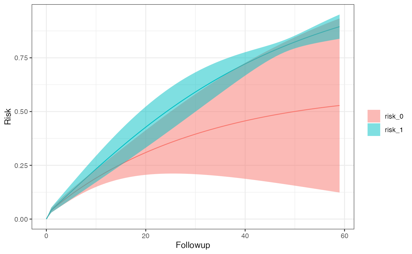
risk_data(model)
#> Index: <Followup>
#>           Method Followup      A      Risk   95% LCI   95% UCI         SE
#>           <char>    <num> <char>     <num>     <num>     <num>      <num>
#> 1: dose-response       60      0 0.5282782 0.1234888 0.9330676 0.20652898
#> 2: dose-response       60      1 0.8949096 0.8385038 0.9513155 0.02877903
risk_comparison(model)
#>    Followup    A_x    A_y Risk Ratio RR 95% LCI RR 95% UCI Risk Differerence
#>       <num> <fctr> <fctr>      <num>      <num>      <num>             <num>
#> 1:       60 risk_0 risk_1  1.6940120  0.7764763   3.695769         0.3666314
#> 2:       60 risk_1 risk_0  0.5903146  0.2705797   1.287869        -0.3666314
#>     RD 95% LCI RD 95% UCI
#>          <num>      <num>
#> 1: -0.07309383 0.80635663
#> 2: -0.80635663 0.07309383
Dose-response with 5 bootstrap samples and losses-to-followup
options <- SEQopts(km.curves = TRUE,
                   bootstrap = TRUE,
                   bootstrap.nboot = 5,
                   # tells SEQuential to expect LTFU as the censoring column
                   cense = "LTFU",
                   # tells SEQuential to treat this column as the
                   # censoring eligibility column
                   cense.eligible = "eligible_cense")

# use example data for LTFU
data <- SEQdata.LTFU
model <- SEQuential(data, id.col = "ID",
                          time.col = "time",
                          eligible.col = "eligible",
                          treatment.col = "tx_init",
                          outcome.col = "outcome",
                          time_varying.cols = c("N", "L", "P"),
                          fixed.cols = "sex",
                          method = "dose-response",
                          options = options)
#>
#> Full dataset: 54,687 observations, 13 variables
#>
#> Non-required columns provided, pruning for efficiency
#>
#> Pruned
#>
#> Original dataset (eligible subjects): 29,624 observations, 10 variables
#>
#> Expanding Data...
#>
#> Pre-filter expansion: 1,609,859 observations
#>
#> Expanded dataset: 1,119,229 observations, 17 variables
#>
#> Expansion Successful
#>
#> Final analysis dataset: 1,119,229 observations, 17 variables
#>
#> Moving forward with dose-response analysis
#>
#> Bootstrapping with 80% of 1,000 subjects (800 subjects, ~895,383 observations per resample) 5 times
#>
#> dose-response model created successfully
#>
#> Creating Survival curves
#>
#> Completed

km_curve(model, plot.type = "risk")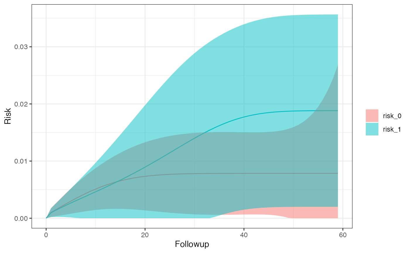
risk_data(model)
#> Index: <Followup>
#>           Method Followup      A        Risk     95% LCI    95% UCI          SE
#>           <char>    <num> <char>       <num>       <num>      <num>       <num>
#> 1: dose-response       60      0 0.007847443 0.000000000 0.02684988 0.009695299
#> 2: dose-response       60      1 0.018827788 0.001997953 0.03565762 0.008586808
risk_comparison(model)
#>    Followup    A_x    A_y Risk Ratio RR 95% LCI RR 95% UCI Risk Differerence
#>       <num> <fctr> <fctr>      <num>      <num>      <num>             <num>
#> 1:       60 risk_0 risk_1  2.3992259 0.44856849  12.832566        0.01098034
#> 2:       60 risk_1 risk_0  0.4168011 0.07792674   2.229314       -0.01098034
#>     RD 95% LCI RD 95% UCI
#>          <num>      <num>
#> 1: -0.01349983 0.03546052
#> 2: -0.03546052 0.01349983
Dose-response with 5 bootstrap samples and competing events
options <- SEQopts(km.curves = TRUE,
                   bootstrap = TRUE,
                   bootstrap.nboot = 5,
                   # Using LTFU as our competing event
                   compevent = "LTFU")

data <- SEQdata.LTFU
model <- SEQuential(data, id.col = "ID",
                          time.col = "time",
                          eligible.col = "eligible",
                          treatment.col = "tx_init",
                          outcome.col = "outcome",
                          time_varying.cols = c("N", "L", "P"),
                          fixed.cols = "sex",
                          method = "dose-response",
                          options = options)
#>
#> Full dataset: 54,687 observations, 13 variables
#>
#> Non-required columns provided, pruning for efficiency
#>
#> Pruned
#>
#> Original dataset (eligible subjects): 29,624 observations, 10 variables
#>
#> Expanding Data...
#>
#> Pre-filter expansion: 1,609,859 observations
#>
#> Expanded dataset: 1,119,229 observations, 16 variables
#>
#> Expansion Successful
#>
#> Final analysis dataset: 1,119,229 observations, 16 variables
#>
#> Moving forward with dose-response analysis
#>
#> Bootstrapping with 80% of 1,000 subjects (800 subjects, ~895,383 observations per resample) 5 times
#>
#> dose-response model created successfully
#>
#> Creating Survival curves
#>
#> Completed

km_curve(model, plot.type = "risk")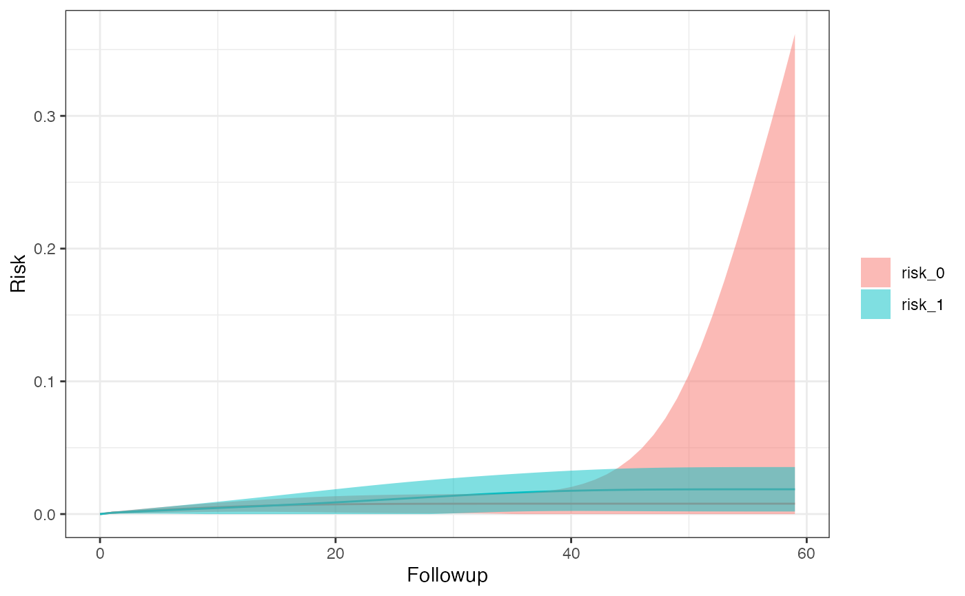
risk_data(model)
#> Index: <Followup>
#>           Method Followup      A        Risk 95% LCI    95% UCI         SE
#>           <char>    <num> <char>       <num>   <num>      <num>      <num>
#> 1: dose-response       60      0 0.007586789       0 0.25972299 0.12864328
#> 2: dose-response       60      1 0.003641046       0 0.02703035 0.01193354
risk_comparison(model)
#>    Followup    A_x    A_y Risk Ratio RR 95% LCI RR 95% UCI Risk Differerence
#>       <num> <fctr> <fctr>      <num>      <num>      <num>             <num>
#> 1:       60  inc_0  inc_1  0.4799192 0.02752717   8.367096      -0.003945743
#> 2:       60  inc_1  inc_0  2.0836841 0.11951578  36.327751       0.003945743
#>    RD 95% LCI RD 95% UCI
#>         <num>      <num>
#> 1: -0.2462717  0.2383802
#> 2: -0.2383802  0.2462717
Dose-response hazard ratio with 5 bootstrap samples and competing events
options <- SEQopts(# km.curves must be set to FALSE to turn on hazard
                   # ratio creation
                   km.curves = FALSE,
                   # set hazard to TRUE for hazard ratio creation
                   hazard = TRUE,
                   bootstrap = TRUE,
                   bootstrap.nboot = 5,
                   compevent = "LTFU")

data <- SEQdata.LTFU
model <- SEQuential(data, id.col = "ID",
                          time.col = "time",
                          eligible.col = "eligible",
                          treatment.col = "tx_init",
                          outcome.col = "outcome",
                          time_varying.cols = c("N", "L", "P"),
                          fixed.cols = "sex",
                          method = "dose-response",
                          options = options)
#>
#> Full dataset: 54,687 observations, 13 variables
#>
#> Non-required columns provided, pruning for efficiency
#>
#> Pruned
#>
#> Original dataset (eligible subjects): 29,624 observations, 10 variables
#>
#> Expanding Data...
#>
#> Pre-filter expansion: 1,609,859 observations
#>
#> Expanded dataset: 1,119,229 observations, 16 variables
#>
#> Expansion Successful
#>
#> Final analysis dataset: 1,119,229 observations, 16 variables
#>
#> Moving forward with dose-response analysis
#>
#> Bootstrapping with 80% of 1,000 subjects (800 subjects, ~895,383 observations per resample) 5 times
#>
#> Completed

# retrieve hazard ratios
hazard_ratio(model)
#> Hazard ratio          LCI          UCI
#>    0.9582143    0.7107252    1.2918841
Dose-response with 5 bootstrap samples and competing events in subgroups defined by sex
options <- SEQopts(km.curves = TRUE,
                   bootstrap = TRUE,
                   bootstrap.nboot = 5,
                   compevent = "LTFU",
                   # define the subgroup
                   subgroup = "sex")

data <- SEQdata.LTFU
model <- SEQuential(data, id.col = "ID",
                          time.col = "time",
                          eligible.col = "eligible",
                          treatment.col = "tx_init",
                          outcome.col = "outcome",
                          time_varying.cols = c("N", "L", "P"),
                          fixed.cols = "sex",
                          method = "dose-response",
                          options = options)
#>
#> Full dataset: 54,687 observations, 13 variables
#>
#> Non-required columns provided, pruning for efficiency
#>
#> Pruned
#>
#> Original dataset (eligible subjects): 29,624 observations, 11 variables
#>
#> Expanding Data...
#>
#> Pre-filter expansion: 1,609,859 observations
#>
#> Expanded dataset: 1,119,229 observations, 16 variables
#>
#> Expansion Successful
#>
#> Final analysis dataset: 1,119,229 observations, 16 variables
#>
#> Moving forward with dose-response analysis
#>
#> Bootstrapping with 80% of 1,000 subjects (800 subjects, ~895,383 observations per resample) 5 times
#>
#> dose-response model created successfully
#>
#> Creating Survival Curves for sex_0
#>
#> Creating Survival Curves for sex_1
#>
#> Completed

km_curve(model, plot.type = "risk")
#> $sex_0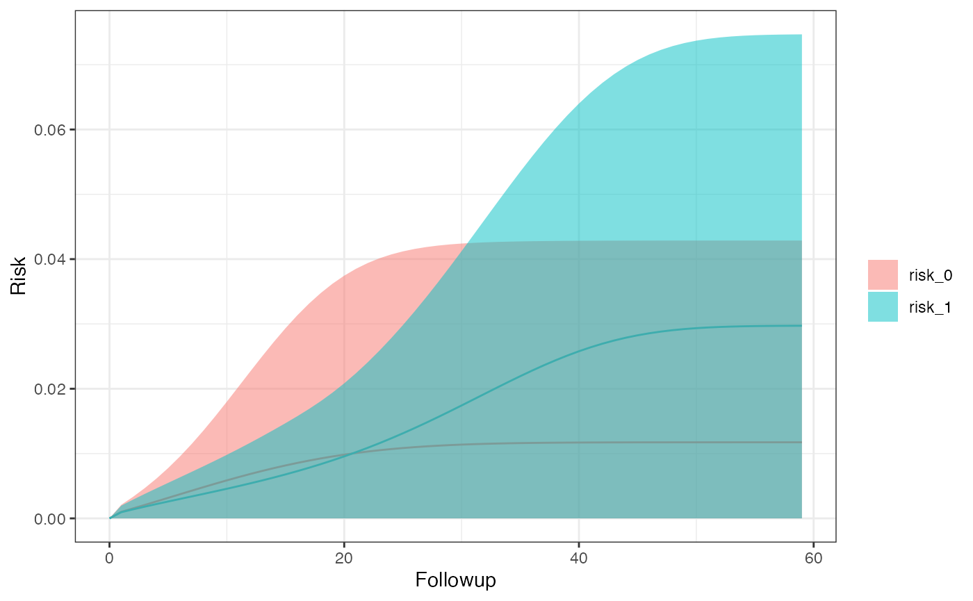
#>
#> $sex_1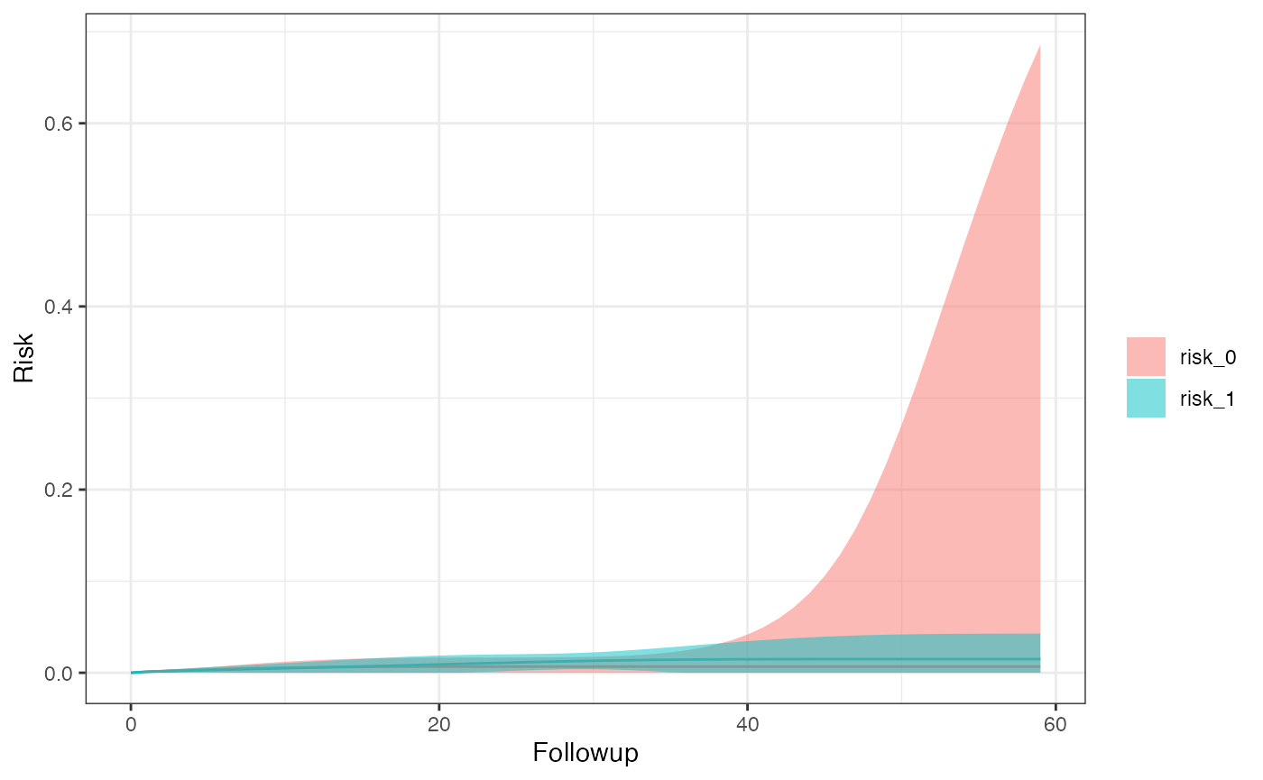
risk_data(model)
#> $sex_0
#> Index: <Followup>
#>           Method Followup      A       Risk 95% LCI    95% UCI         SE
#>           <char>    <num> <char>      <num>   <num>      <num>      <num>
#> 1: dose-response       60      0 0.01125753       0 0.04037235 0.01485477
#> 2: dose-response       60      1 0.01869016       0 0.06423635 0.02323828
#>
#> $sex_1
#> Index: <Followup>
#>           Method Followup      A       Risk 95% LCI    95% UCI         SE
#>           <char>    <num> <char>      <num>   <num>      <num>      <num>
#> 1: dose-response       60      0 0.00659838       0 0.47302574 0.23797751
#> 2: dose-response       60      1 0.01221464       0 0.04936991 0.01895712
risk_comparison(model)
#> $sex_0
#>    Followup    A_x    A_y Risk Ratio   RR 95% LCI RR 95% UCI Risk Differerence
#>       <num> <fctr> <fctr>      <num>        <num>      <num>             <num>
#> 1:       60  inc_0  inc_1  1.6602358 2.459467e-05  112072.36       0.007432626
#> 2:       60  inc_1  inc_0  0.6023241 8.922806e-06   40659.22      -0.007432626
#>     RD 95% LCI RD 95% UCI
#>          <num>      <num>
#> 1: -0.04559720 0.06046245
#> 2: -0.06046245 0.04559720
#>
#> $sex_1
#>    Followup    A_x    A_y Risk Ratio RR 95% LCI RR 95% UCI Risk Differerence
#>       <num> <fctr> <fctr>      <num>      <num>      <num>             <num>
#> 1:       60  inc_0  inc_1  1.8511568 0.09376874   36.54503       0.005616256
#> 2:       60  inc_1  inc_0  0.5402028 0.02736350   10.66454      -0.005616256
#>    RD 95% LCI RD 95% UCI
#>         <num>      <num>
#> 1: -0.4278731  0.4391056
#> 2: -0.4391056  0.4278731